The paper  did not mention output frequency.  The method I used for hbond calculation is for each frame, I calculate all the hbonds, and push the hbond into live_array if the hbonds existed in previous frame still exist in current frame, and push the hbond into dead_array if not. so the total number of appearance in live_array is total number of frames that this hbond is still alive, and the total number of appearance in dead_array is times this hbond had died. The number in live_array divided by number in dead_array is the average life time for that hbond. The simulation of water are running on a 40 box.

**When plot this graph, set width=0.001, because 1step=0.002ps.

The average hbond lifetime is 0.02480.0131 ps, which is way too short, so what is the problem? look the picture below from reference 4.

During simulation,  some hbonds can incidentally go beyond the criterion for 10-20 fs(5-10 steps) , and some honds accidently formed due to duffusion motion. We need to rule out these two situations as much as possible.

there are two ways to improve this, i) change the hbond criteria, ii) develop factors that can adjust the break and reforming of hbond.  let's first change the hbond criteria to Dist=3.5A, Ang=30.

After we change the criteria for hbond, the average hbond lifetime shift to about 0.05510.0323ps, this is still not enough, so we need to try method ii to calculate hbond lifetime. I defined a factor called "break", means if within $break time the hbond comes back, we still consider the hbond never died, and also add another factor called "continue", means if the hbond exist greater than $continue, then we count this as a true hbond.To realize this, I save all hbonds of one frame into hbond_live, but this time I also save the $frame, so hbonds_live={{donor acceptor hydrogen frame}...}, later on I will use this frame to decide the hbond lifetime.

lifetime on top is output frequency=1, and break=1,5,10, continue=1,5,10, the average is 0.05ps, 0.06ps,0.10ps respectively .
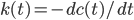
lifetime at the bottom is output frequency=10, the average is 0.05, 0.57 and 0.89. Of cause, we can set the factor to be break=100, continue=100, or even longer, but the problem is if we we use bigger break or continue, we also need to increase sample time, from 1000 steps to 10000 or even longer, this will tremendously increase the calculation time. That is the reason some research step further to study  correlation functions c(t), the probability that one hbond still bonded at time t provided the pair was bonded at t=0(independent of possible breaking in the interim time).

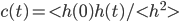
h(t)=1 if bonded, and 0 if not bonded
So P(t) is history dependent, but c(t) is history independent.

And also reactive flux, defined by derivative, which measure the effective decay rate of an initial set of hbonds.

If we only need to care about hbond every 10 steps, when we run the simulation we don't need to spit out energy every step, so 10 steps would be a appropriate setting for energy output frequency, and this will also significantly decrease\

The electric field fluctuations caused by vibration of molecule itself and bonding with neighboring molecules leads to water dissociation.

The thermodynamic property of this process at 25 and 0.1 MPa:

ΔU = 59.5 kJ mol^-1, ΔV =21.4 cm³ mol^-1, ΔH =55.8 kJ mol^-1, ΔG = 79.9 kJ mol^-1, ΔS = -77.2 J K^-1 mol^-1

The dissociation constant of water at 25 Kw is equal to 1.0x10^-14.

The tunneling of hydrogen ions can be described by Grotthuss mechanism:

Hydrogen Ion Diffusion 

Hydroxyl Ion Diffusion   

This process significantly facilitate the movement of hydrogen ion, and it is believed protons move(apparant move) twice as fast as hydroxide ions and seven times as fast as Na⁺. The aboved mechanism is just a simplified scheme of hydrogen ion transfer, the actual situation is much more complex involved different hydroxoniums(H₅O₂⁺,H₇O₃⁺,....).

No matter how protons transfer through "water network" or "water wire", one thing in common is that protons play the role like glue to coordinate between water molecules or water molecules with solute molecules. Some research also noted that excess protons can create their own water wires, and influence proton translocation in biological systems.

Forces here we are talking about is non-bonding interactions, bonding interaction(~100kcal/mol) holds the atoms together as a molecule, non-bonding interaction(~RT=2.5kJ/mol)holds the molecules together in an condensed phase, without this interaction there would be one gaseous state only. All molecular interactions are inherently electrostatic in nature. We classify all interactions to two major categories: (1) strong charge involved interaction to describe formally charged species(ions), (2) weak collectively van der Waals interaction including dipole-dipole,dipole-induced dipole and dispersion to describe partial charged species.

equation    note
ionic interation    ion-ion interaction        
Electrostatic interaction between electrically-charged particles is the strongest of all the non-bonding intermolecular forces, as we learned in school, this force also called coulombic force since it follows Coulomb's Law. The energy level of ionic interaction is 1~20kcal/mol(ionic bond hundreds of kcal/mol).

ion-diopole interation        
diopolar interation        Dipole-Dipole Interaction 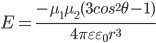       The diple moment of an electron and a proton separated by 1 Å equals 4.8 Debye((4.810-10esu) (10-8cm)=4.810-18 esu cm), the dipole moment of water is 1.85 Debye(gas),2.95Debye(liquid), 3.09 Debye(ich Ih)
Dipole-Induced Dipole Interaction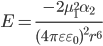        
Dispersion        
other interactions      interaction