Water molecules play significant roles in biological process through interacting with all kinds of solutes, such as proteins, organic compounds and ions. Many research have been performed on the thermal dynamics and kinetics of water molecules in solutions experimentally (infrared spectroscopy,Raman spectroscopy) and computationally (MD). They are so popular and tiny that makes them negligible to the research compared to large and distinct molecules. This study is to investigate the functionalities that water molecules might have on solute molecules through molecular simulation.

The anomalies from water were believed to be connected to the hydrogen bond network in liquid water. We will be studying the hydrogen bond network properties, and investigate how it is influenced by solutes in this network.

Table of Contents

1.Simulation Parameters for Water Molecule and Hydrogen Bond

1.1. Water Molecule

1.2. Hydrogen Bond

2.Simulation Protocol

3.Properties of Hydrogen Bond

3.1.Degree of Hydrogen Bond

3.2.Hydrogen Bond Lifetime

2.Hydrogen Bond Network in Liquid Water

2.1. Hydrogen Bond Lifetime

2.2. Complex Network Analysis

3.Water Bridges

3.1. Water Bridge Calculation

7.Water Network

7.1Pure Water Box Simulation

7.2Protein In Water Simulation

7.2Water Network & Water Bridge

7.2.1 Complex Network Analysis

1.Simulation Parameters for Water Molecule and Hydrogen Bond

1.1 Water Molecule

Water molecule is V-shaped tetrahedrally arranged through sp3-hybridization. The ideal bond angle for perfect tetrahedral structure is 109.5º, but in case of water , the lone pairs are not positioned as they are with covalent bond, so the negative charge is more "evenly smeared out" between these two lines, this effect makes the hydrogen bonding less stringent and more flexible in angles.

The bond length of OH and angle HOH increase as from gaseous state to solid ice state.

	gas	liquid	solid*
r(OH) Å	0.95718	~0.990	~1.01
HOH deg	104.474°	~105.5°	~109.5°

* https://en.wikipedia.org/wiki/Ice_Ih

below are two water models in my research:

	TIP3P	SPC/E
r(OH) Å	0.9572	1.0
HOH deg	104.52	109.47
q(O)	-0.834	-0.8476
q(H)	+0.417	+0.4238

1.2 Hydrogen Bond

Hydrogen bond is NOT just dipole-dipole interaction OR ion-dipole interaction, it is a weak covalent bond in which hydrogen bridges two different molecules, it is a partial covalent bond formation between H and A......, see IUPAC definition of hydrogen bond here.

The mean donor-acceptor distances in protein secondary structure elements are close to 3.0 Å, (Jeffrey). Jeffrey categorizes hbonds with donor-acceptor distances of 2.2-2.5 as "strong, mostly covalent", 2.5-3.2 Å as "moderate, mostly electrostatic", and 3.2-4.0 Å as "weak, electrostatic". Energies are given as 40-15, 14-4, and <4 kcal/mol respectively. Most hydrogen bonds in proteins are in the moderate category.

The parameters vary from their environment, hydrogen bonding, solutes, ions, etc..The molecular simulation employ fixed parameters which is not actual situation in reality, so we need to show some flexibility when we extract and analyze our data. In this research, we choose geometric definition and employ distance of O-H-O as 3.5Å, and angle between 150º~180º.

2. Simulation Protocol

We will be using CHARMM, NAMD and AMBER to run the simulation, the detailed information can be found in their linked pages.

timestep	0.002ps
cutoff	14
NPT	1atm
temp	300K
shake	off

3.Properties of Hydrogen Bond

3.1.Degree of Hydrogen Bond

STEP1: load production trajectory into vmd and calculate all hbonds.

vmd md.psf md.dcd

open tcl console and type:

source ~/toolset/water_bridge.tcl

start_hbonding -water

Hbond information will be saved in ./hbonds_water.txt.

STEP2:Calculate degree of water hbonding.

>source("~/toolset/deg.R")

("watch -n 1 cat tmp" to watch the progress of calculation)

this will save degree information in deg.txt:

0.1626174 0.3690746 0.313681 0.1305475 0.02332362 0.0007558579 0

.....

every line indicate average frequency of 0,1,2,3,4,5,6 hydrogen bonds in one frame.

now, we plot the degree of hbonding:

z<-read.table("deg.txt")

z.means<-colMeans(z)

df=data.frame(z.means)

df$degree<-c(0,1,2,3,4,5,6,7)

ggplot(df,aes(x=degree,y=z.means))+geom_bar(stat="identity",fill="red")+theme_bw()+xlab("degree of hydrogen bonding")+ylab("fraction")+theme(axis.text=element_text(size=20),axis.title=element_text(size=24,face="bold"))+scale_x_continuous(breaks=c(0,1,2,3,4,5,6,7))

library(data.table)

library(ggplot2)

library(RColorBrewer) #display.brewer.all() to see all color palettes

filelist<-c("./Pure_9261/deg.txt","./NaCl_1/deg.txt","./Na20Cl20/deg.txt","./Mg20Cl40_1/deg.txt","./Al20Cl60_1/deg.txt","./Na650Cl650/deg.txt","./Na1300Cl1300/deg.txt")

temp <- lapply(filelist, fread, sep=" ")

data<-melt(mapply(c, colMeans(temp[[1]]), colMeans(temp[[2]]),colMeans(temp[[3]]),colMeans(temp[[4]]),colMeans(temp[[5]]),colMeans(temp[[6]]),colMeans(temp[[7]])))

for (i in 1:nrow(data)) {if (data$Var1[i] ==1) {data$Var1[i]<-"Pure_9261"} else if (data$Var1[i] == 2) {data$Var1[i]<-"NaCl"} else if (data$Var1[i] == 3) {data$Var1[i]<-"Na20Cl20"} else if (data$Var1[i] ==4) {data$Var1[i]<-"Mg20Cl40"} else if (data$Var1[i] == 5) {data$Var1[i]<-"Al20Cl60"} else if (data$Var1[i] == 6) {data$Var1[i]<-"Na650Cl650"} else if (data$Var1[i] == 7) {data$Var1[i]<-"Na1300Cl1300"} }

for (i in 1:8) {nam<-paste("V",i,sep="");levels(data$Var2)[levels(data$Var2)==nam]<-i}

data$Var1<-factor(c("Pure_9261","NaCl","Na20Cl20","Mg20Cl40","Al20Cl60","Na650Cl650","Na1300Cl1300"),levels=c("Pure_9261","NaCl","Na20Cl20","Mg20Cl40","Al20Cl60","Na650Cl650","Na1300Cl1300"))

ggplot(data,aes(x=Var2,y=value,fill=Var1))+geom_bar(stat="identity",position="dodge")+labs(title="Comparison of Degree of HBonds",x="Degree of HBonds",y="Frequency")+theme(axis.title=element_text(size=20),axis.text=element_text(size=12),legend.key.size=unit(2.5,"cm"),legend.title=element_blank(),plot.title=element_text(size=30))+scale_fill_brewer(palette = "Greens")

As we see from graph above, the degree of hbonds in bulk water show a normal distribution like pattern, the pattern was altered by adding ions into it. Adding ions into the the box significantly increase the population of hydrogen bonds with less degree, while decreasing the population of hydrogen bonds with higher degree except Mg ion which show a similar pattern as bulk water. The high the concentration the distribution shift to less degree of hydrogen bonds.

2.2.Hydrogen Bond Lifetime

One factor of dynamics of H-bond network is hydrogen bond lifetime,The relaxation time for water dipole reorientation at room temperature is about 10ps, the average hydrogen bond lifetime will roughly agree with (or smaller than) this value because reorientation is impossible without breaking at least one hbond. The picture below is calculation of average hbond lifetime () from reference 5. and 8.

( is the mean of the distribution of hbond lifetime P(t), which measures the probability that an initially bonded pair remains bonded at all times up to time t, and breaks at t. P(t) is obtained from simulations by building a histogram of hbond lifetimes for each configuration, .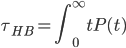

In this research, for simplicity, we just calculate the discontinuous hbond lifetime, that is we sum up all times that a certain hydrogen bond spans over the whole trajectory no matter continuous or discontinuous in between.

Amber simulation of Pure water and water with salt in it can be found here.

Pure_6859(6859 water molecules)

Pure_8000(8000 water molecules)

Pure_9261(9261 water molecules)

NaCl(9259 water molecules, 1 Na+, 1 Cl-, 27779 atoms total,~0.007M)

Na20Cl20(9221 water molecules,20 Na+, and 20 Cl-,27703 atoms total,~0.13M)

Mg20Cl40(9261 water molecules,20 Mg2+, and 40Cl-, 27663 atoms total,~0.13M)

Al20Cl60(9181 water molecules, 20 Al3+, and 60 Cl-, 27623 atoms total, ~0.13M)

Na650Cl650(7961 water molecules, 650 Na+, 650 Cl-,25183 atoms total,~4.1M)

Na1300Cl1300(6661 water molecules, 1300 Na+, 1300 Cl-,22583 atoms total, ~8.2M)

Amber simulation of "TOP100" proteins can be found here. To study the influence of proteins on hydrogen bond network, we performed molecular simulation of 96 proteins from dynameo benchmark, each protein was downloaded from PDB data bank, and only amino residues were kept, and blocked by ACE and NME at the N-terminal and C-terminal respectively.

Following are steps to analyze the lifetime(discontinuous) of hydrogen bonds in pure water and salt solutions, run the same commands in each directory:

vmd water_box.prmtop -netcdf md.mdcrd

(delete beginning 9000 frames by choosing last=8999, we will only analyze last 1000 frames)

tcl/tk windows:

source ~/toolset/water_bridge.tcl

start_hbonding -water -residence

bash shell:

residence4.pl hbonds_residence_all.txt [name_of_system] 1

copy loophbond.sh loophbond.tcl to ./TOP100.

./loophbond.sh

./loopresidence4R.sh

cat *_hbonds_residence_all_R.txt>tmp.txt

awk '{$1="protein";print $0}' tmp.txt > protein_hbonds_residence_all_R.txt

closeAllConnections()

rm(list=ls())

library(data.table)

library(ggplot2)

filelist<-c("./Pure_6859/hbonds_residence_all_R.txt","./Pure_8000/hbonds_residence_all_R.txt","./Pure_9261/hbonds_residence_all_R.txt","./NaCl_1/hbonds_residence_all_R.txt","./Na20Cl20_1/hbonds_residence_all_R.txt","./Mg20Cl40_1/hbonds_residence_all_R.txt","./Al20Cl60_1/hbonds_residence_all_R.txt","./Na650Cl650/hbonds_residence_all_R.txt","./Na1300Cl1300/hbonds_residence_all_R.txt","../../../work2/TOP100/protein_hbonds_residence_all_R.txt")

temp <- lapply(filelist, fread, sep=" ")

data<-melt(temp)

Na1300<-subset(data,V1=='Na1300Cl1300')

Na650<-subset(data,V1=='Na650Cl650')

rest<-subset(data,V1!='Na650Cl650' & V1!='Na1300Cl1300')

medx_Na1300<-median(Na1300$value)

medx_Na650<-median(Na650$value)

medx_rest<-median(rest$value)

ggplot(data,aes(x=value,colour=V1,fill=V1))+geom_density(alpha=0)+scale_colour_manual(values=c("black","black","red","black","green","black","blue","black","black","black"))+xlim(0,100)+theme(axis.title=element_text(size=20),axis.text=element_text(size=12),legend.key.size=unit(2.5,"cm"),legend.title=element_blank(),plot.title=element_text(size=30))+labs(title="lifetime of HBonds",x="steps(in hundreds)")+geom_vline(xintercept=medx_Na1300,colour="red",linetype="longdash")+geom_vline(xintercept=medx_Na650,colour="green",linetype="longdash")+geom_vline(xintercept=medx_rest,colour="black",linetype="longdash")+annotate("text",x=9,y=0.01,label="10",angle=90)+annotate("text",x=11,y=0.01,label="12",angle=90)+annotate("text",x=15,y=0.01,label="15",angle=90)

As we see from the graph above,majority of hbonds lasts within 5000 steps which is 10ps, the average lifetime for most system except Na1300Cl1300 and Na560Cl650 is about 10 steps(=10*0.002ps=0.02ps), while the average lifetime for Na1300Cl1300 and Na560Cl650 are 12 steps (12*0.002ps=0.024ps) and 16 steps (16* 0.002ps=0.036ps) respectively. As the ionic strength increase, the distribution of lifetime shift to longer life time, which means the existence of ions in solution extend the lifetime of hbonds. Since this is statistics about whole box of waters, a very small portion of ions will not significantly change the lifetime of hydrogen bonds of most water molecules inside the box, and obviously the existence of protein will not influence the lifetime of hydrogen bonds in bulk water as well.

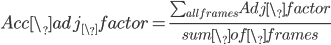
To further invesigate the influence of solutes to hbonds lifetime, we need to take closer look at hydrogen bonds which are adjacent to solute molecules. To realize this, we invent a variale called adjacent factor, which takes the form of equation below:

in which:

0<base# <1

distance_to_# is the shortest distance from hbond donor to the terminal carbon atoms of classified groups which shows in the table below:

name   description
cations   AL,MG,NA
ions   CL
protein_A   Aminoacids with Positively Charged Side Chain:Arg,His or HIE,Lys
protein_B   Aminoacids with Negtively Charged Side Chain:Asp,Glu
protein_C   Aminoacids with Polar Uncharged Side Chain:Ser,Thr,Asn,Gln
protein_D   Special Cases:Cys,Gly,Pro
Protein_E   Aminoacids with Hydorphobic Side Chain:Ala,Ile,Leu,Met,Phe,Trp,Tyr,Val
Accumulated adjacent factor:

"It appears that although the occupancy and residence times of the majority of sites are rather bulk-like, the residence time distribution is shifted toward the longer components, relative to bulk. The sites with particularly long residence times are located only in the cavities and clefts of the protein. This indicates that other factors, such as hydrogen bonds and hydrophobicity of underlying protein residues, play a lesser role in determining the residence times of the longest-lived sites." (7)

filelist<-c("./Pure_9261/Pure9261_hbonds_water_residence.txt","./NaCl_1/NaCl_hbonds_water_residence.txt","./Na20Cl20_1/Na20Cl20_hbonds_water_residence.txt","./Mg20Cl40_1/Mg20Cl40_hbonds_water_residence.txt","./Al20Cl60_1/Al20Cl60_hbonds_water_residence.txt","./Na650Cl650/Na650Cl650_hbonds_water_residence.txt","./Na1300Cl1300/Na1300Cl1300_hbonds_water_residence.txt")

temp <- lapply(filelist, fread, sep=",",select=4:5)

data<-melt(temp,id.vars='V4')

data$L1<-as.character(data$L1)

ggplot(data,aes(x=V4,y=value,color=L1))+geom_point()+scale_colour_manual(values=c("red","yellow","orange","gray","green","blue","black"))

2.Hydrogeon Bond Network in Liquid Water

Hydrogen bonded networks play an important role in determining the physical properties of many molecular liquids and solids, and play a crucial role in the structure and fuction of most biomolecules, Among these, water is the most extensively studied molecule.(6,13,14) First Paper I found talk about water network in liquid water is ref.10, this paper discuss the distribution of non-short-circuited hydrogen-bond polygons. This hydrogeon bond network become complicated due to the variety ionization form of water molecules. The hydrogen ion must exist as ions with formula H₃O+(H₂O)n, H₃O+(hydroxonium ion, hydronium ion is obsolete) H₅O₂+ H₉O₄+ H₁₃O₆+. Below are some popular hydrogen ions and hydroxide ions.

formula	structure	notes
H₃O+		H₃O+ can donate three hydrogen bonds and accept almost none, the strength of these donated hydrogen bonds being over twice as strong as those between H₂O molecules in bulk water. The presence of an H₃O+ ion influence at least 100 surrounding water molecules.
H₅O₂+		Two H₅O₂+ dihydronium ions with top one has a asymmetrical proton and bottom one has a symmetric proton.
H₉O₄+		H₉O₄⁺ formed by attach a water molecule on each side of H₅O₂⁺, allows the shuttling of protons between the four molecules.
H₁₃O₆+		H₁₃O₆+ formed by fully hydration of H₅O₂+. The bottom one is more stable(~1kJmol^-1).
OH-		Hydroxide ions are molecular ions with the formula OH-, formed by the loss of a proton from a water molecule
H₃O₂-		The hydroxide ion (OH-) is a very good acceptor of hydrogen bonds, with the first water molecule binding strongly to form H₃O₂-

The dynamics of the H-bond network of water is believed to play a key role in many processes in physics, chemicstry, and biology. Experiments(depolarized rayleigh scattering, quasi-elastic incoherent neutron scattering) and MD simulation were employed to study the lifetime of H-bonds(9).

2.2. Complex Network Analysis

"In the context of network theory, a complex network is a graph (network) with non-trivial topological features—features that do not occur in simple networks such as lattices or random graphs but often occur in graphs modelling of real systems. "(https://en.wikipedia.org/wiki/Complex_network). The reason we perform complex network analysis on water network is to seek if there is any "non-trivial" substructures in water network which makes water unique thus become the popular solvent for biological processes.

The most popular network analysis tools include:

1.Boost Graph Library（BGL）http://www.boost.org/doc/libs/1_42_0/libs/graph/

2.QuickGraph http://www.codeplex.com/quickgraph

3.igraph http://igraph.sourceforge.net/

4.NetworkX http://networkx.lanl.gov/

Here we perform water network analysis by igraph in R.

STEP1: load trajectory into vmd and calculate hbond pairs, skip to step2 if this has already been done.

vmd md_npt.psf skip10000.dcd

open tcl console and type:

source ~/toolset/water_bridge.tcl

start_hbonding -water

This will save hbond information in ./current directory/hbonds_all.txt.

subset(data,L1=="7" & variable=="V1")

z<-read.table("deg.txt")

z.means<-colMeans(z) or apply(z,2,mean)
error.bar <- function(x, y, upper, lower=upper, length=0.1,...){

+if(length(x) != length(y) | length(y) !=length(lower) | length(lower) != length(upper))

+stop("vectors must be same length")

+arrows(x,y+upper, x, y-lower, angle=90, code=3, length=length, ...)

z.sd<-apply(z,2,sd)

barx<-barplot(z.means,names.arg=0:7,axis.lty=1,ylim=c(0,0.5),xlab="number of hbonds",ylab="density",font.lab=2,cex.lab=2,col="red",main="hbonds of 100 frames(skip 10000)",cex.main=2)

error.bar(barx,z.means,z.sd)

3. Water Bridges

3.1. Water Bridges Calculation

Water as a popular solvent plays a key role in biological reactions, for example protein folding and protein recoganition. The mechanism of these process has not been fully understood yet, a lot of focus has been given to protein as a big solute molecule, and shed much less light on this abundant and small molecule. In this part we will investigate the role of water molecules in stabilizing folded protein and to explore the characteristics of water bridge. Compared to direct hydrogen bond, interactions through water bridges are considered to be more weak, and the contribution of direct hydrogen bonds between amino residues to gibbs free energy to be around 25 kJ mol^-1, the contribution of indrect hydrogen bond through one water molecule is about -10.5kJ mol-1, (page 248, ref. 18.).

In this study, I wrote a vmd script(water_bridge.tcl) to find all hydrogen bond information, then calculate water bridges that span over amino residues along the trajectory. Here we only calculate water bridge up to 3 water bridges for the sake of saving calculation time.

copy loophbondbridge.sh loophbondbridge.tcl to ./work2/TOP100/

./loophbondbridge.sh

this will generate *_bhonds_bridge.txt & *_hbonds_bridge_residence.txt

the formats of *_hbonds_bridge_residence.txt is:

atom index, atom index, atom name, atom name, residue name,residue name, resid, resid, backbone type(BB,BS,SB,SS),frames,total number of frames, bridge score

6,842,N,OG,ALA,SER,2,54,BS,3 5 8,3,0.125

*bridge score:

direct HB:1.0

one water bridge:0.5

two water bridge:0.25

three water bridge:0.125.

final bridge score = sum of bridge score/total frames that bridge exists

library(data.table)

filelist<-list.files(path=".",pattern="*_hbonds_bridge_residence.txt")

temp <- lapply(filelist, fread, sep=",",select=c(9,11))

data<-melt(temp)

tmp1<-aggregate(value~V9,data,sum)

names(tmp1)<-c("type","frame_sum")

tmp1$frequency<-tmp1$frame_sum/(sum(data$value))

tmp1[2,2:3]<-tmp1[2,2:3]+tmp1[3,2:3]

tmp1[2,1]<-"BS/SB"

tmp2<-tmp1[rownames(tmp1) != "3",]

type frame_sum frequency
1 BB 652440 0.3797902
2 BS/SB 613165 0.3569279
4 SS 452291 0.2632819

~~ggplot(tmp2,aes(x=type,y=frequency))+geom_bar(stat="identity",fill="red")+labs(title="Frequency of HBonds Type",x="hbonds type")~~

postscript("frequency_of_hydrogen_bond_type.eps",onefile=FALSE,horizontal=FALSE,paper="special",width=5,height=5)

ggplot(tmp2,aes(x=type,y=frequency))+geom_bar(stat="identity",fill="red")+labs(x="bridge type",y="frequency density")

dev.off()

Above is the frequency of appearing of hbonds between backbone and sidechain. As we can see, backbone to backbone are a little bit more popular than backbone sidechain and sidechain sidechain has least population.

library(data.table)

filelist<-list.files(path=".",pattern="*_hbonds_bridge_residence.txt")

temp <- lapply(filelist, fread, sep=",",select=c(9,12))

data<-melt(temp)

tmp1<-aggregate(value~V9,data,sum)

names(tmp1)<-c("type","score_sum")

~~tmp1[2,2:3]<-tmp1[2,2:3]+tmp1[3,2:3]~~

tmp1[2,2] <- tmp1[2,2]+tmp1[3,2]

tmp1[2,1]<-"BS/SB"

tmp1$average_score[tmp1$type=="BB"]<-tmp1$score_sum[tmp1$type=="BB"]/(nrow(data[data$V9=="BB",]))

tmp1$average_score[tmp1$type=="BS/SB"]<-tmp1$score_sum[tmp1$type=="BS/SB"]/(nrow(data[data$V9=="SB",])+nrow(data[data$V9=="SB",]))

tmp1$average_score[tmp1$type=="SS"]<-tmp1$score_sum[tmp1$type=="SS"]/(nrow(data[data$V9=="SS",]))

tmp2<-tmp1[rownames(tmp1) != "3",]

type score_sum average_score
1 BB 18326.82 0.4619003
2 BS/SB 29170.66 0.4026538
4 SS 19203.35 0.3504069

Above is average bridge score of each type, backbone tend to form direct hydrogen bond and less water bridge than side chain.

temp <- lapply(filelist, fread, sep=",",select=c(5,6,12))

data<-melt(temp)

tmp1<-aggregate(data$value,by=list(data$V5,data$V6),sum)

source("residue_residue_bridge.R")

#!/usr/bin/Rscript\
df<-{}
df<-data.frame(RESI1=character(0),RESI2=character(0),value=numeric(0))
for (i in 1:nrow(tmp1)) {
print(i)
a<-0
if(tmp1[i,1]==tmp1[i,2]) { df<-rbindlist(list(df,as.list(c(tmp1[i,1],tmp1[i,2],tmp1[i,3]))))
} else {
for (j in 1:nrow(tmp1)) {
if((tmp1[i,1]==tmp1[j,2])&(tmp1[i,2]==tmp1[j,1])&(tmp1[i,1] df<-rbindlist(list(df,as.list(c(tmp1[i,1],tmp1[i,2],sum(tmp1[i,3],tmp1[j,3])))))
a<-1
break
} else if ((tmp1[i,1]==tmp1[j,2])&(tmp1[i,2]==tmp1[j,1])&(tmp1[i,1]>tmp1[i,2])) {
a<-1
break
} else {

}
}
if (a==0) {df<-rbindlist(list(df,as.list(c(tmp1[i,1],tmp1[i,2],tmp1[i,3]))))}
}
}

library(ggthemes)

theme_set(theme_solarized())

df$value<-as.numeric(as.character(df$value))

d<-transform(df,new=round(value/5250.5,digits=2))

levels(df$RESI1)<-list("ALA"="ALA","ARG"="ARG","ASN"="ASN","ASP"="ASP","CYS"="CYS","CYX"="CYX","GLN"="GLN","GLU"="GLU","GLY"="GLY","HID"="HID","HIE"="HIE","HIP"="HIP","ILE"="ILE","LEU"="LEU","LYS"="LYS","MET"="MET","PHE"="PHE","PRO"="PRO","SER"="SER","THR"="THR","TRP"="TRP","TYR"="TYR","VAL"="VAL")

levels(df$RESI2)<-list("ALA"="ALA","ARG"="ARG","ASN"="ASN","ASP"="ASP","CYS"="CYS","CYX"="CYX","GLN"="GLN","GLU"="GLU","GLY"="GLY","HID"="HID","HIE"="HIE","HIP"="HIP","ILE"="ILE","LEU"="LEU","LYS"="LYS","MET"="MET","PHE"="PHE","PRO"="PRO","SER"="SER","THR"="THR","TRP"="TRP","TYR"="TYR","VAL"="VAL")

ggplot(data=d,aes(x=RESI1,y=RESI2,fill=new)) + geom_tile()+geom_text(aes(RESI1,RESI2,label = new), color = "#073642", size = 4)+scale_fill_gradient(name=expression("scale"), low = "#fdf6e3", high = "steelblue",breaks=seq(0, 1, by = 0.1),limits = c(0.0, 1.0))

6.Hydrophobic Effect

7.Water Network

Hydrogen bonded networks play an important rold in determining the phsical properties of many molecular liquids and solids, and play a crucial role in the structure and fuction of most biomolecules, Among these, water is the most extensively studied molecule.(6) First Paper I found talk about water network in liquid water is ref.10, this paper discuss the distribution of non-short-circuited hydrogen-bond polygons.

The hydrogen ion can not survive alone in the solution, it must exist as ions with formula H3O+(H2O)n, H3O+(hydroxonium ion, hydronium ion is obsolete) H5O2+ H9O4+ H13O6+ H3O+ can donate three hydrogen bonds and accept almost none, the strength of these donated hydrogen bonds being over twice as strong as those between H2O molecules in bulk water. The presence of an H3O+ ion influence at least 100 surrounding water molecules.

7.1Pure Water Box Simulation

We will perform water simulation by using charmm,namd and amber14 for comparison.

/home/zwei/work/MD/WATERBOX_charmm/

/home/zwei/work/MD/WATERBOX_namd/

/home/zwei/work/MD/WATERBOX_amber/

A water box which has 9261 water molecules will be created by charmm:

charmm < water.inp (http://gene.bio.jhu.edu/charmmscripts/waterbox.inp)

This will creat a water box which has 21*21*21=9261 water molecules. output files:water_box.pdb/crd.

Next we minimize the system and then slowly heating the water box from 50K to 300K.

mpirun -np 12 charmm < heat_euqi_nvt.inp

*CHARMM
*

!open unit 1 card name /home/zwei/softwares/c37a2/toppar/top_all27_prot_na.rtf
open unit 1 card name /share/apps/charmm_c37a2/toppar/top_all27_prot_na.rtf
read rtf card unit 1
close unit 1
!open unit 1 card name /home/zwei/softwares/c37a2/toppar/par_all27_prot_na.prm
open unit 1 card name /share/apps/charmm_c37a2/toppar/par_all27_prot_na.prm
read para card unit 1
close unit 1

open unit 1 card name water_box.pdb
read sequ pdb unit 1
gene WAT first none last none setup warn noangle nodihe
rewind unit 1
read coor pdb unit 1
close unit 1
crystal define cubic 60.0 60.0 60.0 90.0 90.0 90.0
crystal build cutoff 12.0
image byres sele all end

mini sd nprint 10 inbfreq -1 nstep 1000
mini abnr nstep 10000 nprint 10 lattice

open unit 11 write file name heat_equi.dcd

shake bonh
dyna start timestep 0.002 nstep 20000 firstt 50.0 finalt 300.0 teminc 50.0 -
iasors 0 nsavc 10 nsavv 0 nsavq 0 nsavx 0 ntrfrq 200 ieqfrq 100 nprint 10 iprfrq 1000 ihtfrq 1000 inbfrq -1 ihbfrq -1 imgfrq -1 ixtfrq 1000 ichecw 1 -
ewald pmewald kappa 0.32 order 6 fftx 60 ffty 60 fftz 60 -
iuncrd 11 -
echeck 20 iseed random

open unit 1 write card name heat_equi.psf
write psf card unit 1
*PSF
*

open unit 1 write card name heat_equi.crd
write coor card unit 1
*CRD
*

open unit 1 write card name heat_equi.pdb
write coor pdb unit 1
*PDB
*
stop

Then we perform NPT equilibration on the system:

*CHARMM
*

open unit 1 card name /home/zwei/softwares/c37a2/toppar/top_all27_prot_na.rtf
read rtf card unit 1
close unit 1
open unit 1 card name /home/zwei/softwares/c37a2/toppar/par_all27_prot_na.prm
read para card unit 1
close unit 1

open unit 1 card name heat_equi.pdb
read sequ pdb unit 1
gene WAT first none last none setup warn noangle nodihe
rewind unit 1
read coor pdb unit 1
close unit 1

crystal define cubic 64.0 64.0 64.0 90.0 90.0 90.0
crystal build cutoff 12.0
image byres sele all end
shake bonh

!mini abnr nstep 1000 nprint 100 lattice

open unit 11 write file name md_npt.dcd

dyna cpt start timestep 0.002 nstep 1000000 -
iasors 0 nsavc 1 nsavv 0 nsavq 0 nsavx 0 ntrfrq 1000 nprint 100 iprfrq 1000 inbfrq -1 ihbfrq -1 imgfrq -1 ixtfrq 1000 ichecw 1 -
ewald pmewald kappa 0.32 order 6 fftx 64 ffty 64 fftz 64 -
pconstant pmass 400.0 pref 1.0 pgamma 20.0 -
tbath 300.0 tcons hoover reft 300.0 tmass 1000.0 -
iuncrd 11 -
echeck -1 iseed random

open unit 1 write card name md_npt.psf
write psf card unit 1
*PSF
*

open unit 1 write card name md_npt.crd
write coor card unit 1
*CRD
*

open unit 1 write card name md_npt.pdb
write coor pdb unit 1
*PDB
*
stop

Here we set nsavc=1, which is smaller than normally set values(50,100), This simulation will create ~300G trajectory file which inlude 2 ns of NPT pute water box simulation.

We can use catdcd to extract whatever frames we want to analyze from the original trajectory:

example: extract last 10000 frames:

catdcd -o last10000.dcd -first 990001 md_npt.dcd.

or 100 frames by skiping 10000 frames:

catdcd -o skip10000.dcd -stride 10000 md_npt.dcd

namd input configuration file:

# input
coordinates water_box.pdb
structure water_box.psf
parameters /usr/local/lib/vmd/plugins/noarch/tcl/readcharmmpar1.2/par_all27_prot_lipid_na.inp
paratypecharmm on

# Temperature control
set temperature 300
temperature $temperature

# output
set output water_box
outputname $output
dcdfile ${output}.dcd
xstFile ${output}.xst
dcdfreq 100
xstFreq 100
binaryoutput no
binaryrestart no
outputEnergies 100
restartfreq 1000

# Basic dynamics
exclude scaled1-4
1-4scaling 1
COMmotion no
dielectric 1.0
rigidBonds all

# Simulation space partitioning
switching on
switchdist 9
cutoff 10
pairlistdist 12

#PBC
cellBasisVector1 64 0 0
cellBasisVector2 0 64 0
cellBasisVector3 0 0 64
CellOrigin 0. 0. 0.
wrapWater on

#PME
PME on
PMEGridSpacing 1

#Constant Pressure
useGroupPressure yes langevinPiston on
langevinPistonTarget 1.01325
langevinPistonPeriod 100.
langevinPistonDecay 50.
langevinPistonTemp $temperature

# Multiple timestepping
firsttimestep 0
timestep 1
stepspercycle 20
nonbondedFreq 2
fullElectFrequency 4

# Scripting
run 1000000

Amber input scripts:

Minimization:

Minimization of water box
&cntrl
imin = 1, ! Turn on minimization
ncyc=1000, ! If ncyc<maxcyc steepest descent before switching to conjugated gradient for remaining
maxcyc = 5000, ! Total number of minimization cycles
cut = 8, ! Nonbonded cutoff in angstroms
ntpr=100, ! Print frequency
/

pmemd.cuda -O -i min.mdin -o min.out -c water_box.inpcrd -p water_box.prmtop -r min.rst

Heating:

heating and equilibrating
&cntrl
imin=0, irest=0, ntx=1,ntxo=2,
ntpr=100, ntwx=100, nstlim=20000,
dt=0.002, ntt=3, tempi=50.0,
temp0=300, gamma_ln=5.0, ig=-1,
ntc=2, ntf=2, cut=8, iwrap=1,
ioutfm=1,ntrelax=100,
/
&wt type='TEMP0', istep=50.0,istep2=5000,value1=0.0,value2=300.0 /
&wt type='TEMP0', istep=5001,istep2=20000,value1=300.0,value2=300.0 /
&wt type='END' /

pmemd.cuda -O -i heat.mdin -o heat.out -c min.rst -p water_box.prmtop -r heat.rst

Production Run:

Explicit solvent production run
&cntrl
imin=0, irest=1, ntx=5,ntxo=2,
ntpr=100, ntwx=100, nstlim=1000000,
dt=0.002, ntt=3,ntp=1,
temp0=300, gamma_ln=5.0, ig=-1,
ntc=2, ntf=2, cut=8, iwrap=1,
ioutfm=1,ntrelax=100,
/

mpirun -np 2 pmemd.cuda.MPI -O -i md.mdin -o md.out -c heat.rst -p water_box.prmtop -r md.rst -x md.mdcrd

7.2 Protein In Water Simulation

7.2.1 1E0Q

/home/zwei/work/MD/1E0Q/amber

pdb4amber --model=1 --noter -i 1E0Q.pdb -o tmp.pdb

edit tmp.pdb(acetylation ACE and amidation NME)

move H3 to top of the file and replace H3 to C and residue name to ACE.

ATOM 11 H3 MET A 1 -14.434 0.885 -2.035 1.00 0.00 H

ATOM 11 C ACE A 1 -14.434 0.885 -2.035 1.00 0.00 C

&& move atom OXT from last residue to bottom of the file and replace OXT to N, residue name to NME

ATOM 276 OXT VAL A 17 -14.136 -2.108 2.130 1.00 0.00 O

ATOM 276 N NME A 17 -14.136 -2.108 2.130 1.00 0.00 N

tleap -f tleap.in

mpirun -np 12 pmemd.MPI -O -i min.mdin -c 1e0q_box.inpcrd -p 1e0q_box.prmtop -r min.rst

pmemd.cuda -O -i heat.mdin -o heat.out -c min.rst -p 1e0q_box.prmtop -r heat.rst -x heat.mdcrd

mpirun -np 2 pmemd.cuda.MPI -O -i md.mdin -o md.out -c heat.rst -p 1e0q_box.prmtop -r md.rst -x md.mdcrdmpirun -np 2 pmemd.cuda.MPI -O -i md.mdin -o md.out -c heat.rst -p 1e0q_box.prmtop -r md.rst -x md.mdcrd

TOP100 proteins bechmark:

copy loopwaterbridge.tcl, loop.sh, pipeline.sh to ./TOP100,

pipeline.sh(to prepare and generate trajectories)

loop.sh(to analyze the last 100 frames, and generate *_bridge_residence.txt *_bridges.txt)

7.2Water Network & Water Bridge

Water is a so common but most fascinating substances in the universe(12). It possesses a number of anomalous properties(high melting and boiling points relative to water's small molecular weight, water's expansion of volume upon freezing). All of the anomalous properties of water are connected to the fact that water forms an extensive hydrogen-bond network.

7.2.1 Complex Network Analysis

The most popular network analysis tools include:

1.Boost Graph Library（BGL）http://www.boost.org/doc/libs/1_42_0/libs/graph/

2.QuickGraph http://www.codeplex.com/quickgraph

3.igraph http://igraph.sourceforge.net/

4.NetworkX http://networkx.lanl.gov/

Here we use igraph in R to analyze the water network structure.

STEP1: load trajectory into vmd and calculate hbond pairs

vmd md_npt.psf skip10000.dcd

open tcl console and type:

source ~/toolset/water_bridge.tcl

start_hbonding -water

This will save hbond information in ./current directory/hbonds.txt with the format as follows,

0 25443 18441

....

*0 is the frame number,

255443 and 18443 are index of water oxygens.

STEP2:Calculate degree of water hbonding.

>source("deg.R")

#!/usr/bin/Rscript\
library(igraph)
rm(list=ls())
if(file.exists("deg.txt")){file.remove("deg.txt")}
for (i in seq(from=0,to=99,by=1)) {
name<-paste0("g",(i))
name1<-paste0("net",(i))
  name2<-paste0("deg",(i))
  name3<-paste0("H",(i))
  write(i,file="tmp")
assign(name,read.table(pipe("awk -v var=`cat tmp` '{if ($1==var) print $2,$3}' hbonds.txt")))
  assign(name1,graph_from_data_frame(eval(as.symbol(name)),directed=F))
  for (j in seq(0,27781,by=3)) {if(!j %in% V(eval(as.symbol(name1)))$name) {assign(name1,add_vertices(eval(as.symbol(name1)),1,name=j))}}
  assign(name2,degree(eval(as.symbol(name1)),mode="all"))
  assign(name3,hist(eval(as.symbol(name2)),plot=FALSE,breaks=c(-0.5,0.5,1.5,2.5,3.5,4.5,5.5,6.5,7.5)))
  write(eval(as.symbol(name3))$density,file="deg.txt",append=TRUE,ncolumns=8)

("watch -n 1 cat tmp" to watch the progress of calculation)

this will save degree information in deg.txt:

0.1626174 0.3690746 0.313681 0.1305475 0.02332362 0.0007558579 0

.....

every line indicate average frequency of 0,1,2,3,4,5,6 hydrogen bonds in one frame.

now, we plot the degree of hbonding:

z<-read.table("deg.txt")

z.means<-colMeans(z) or apply(z,2,mean)
error.bar <- function(x, y, upper, lower=upper, length=0.1,...){

+if(length(x) != length(y) | length(y) !=length(lower) | length(lower) != length(upper))

+stop("vectors must be same length")

+arrows(x,y+upper, x, y-lower, angle=90, code=3, length=length, ...)

z.sd<-apply(z,2,sd)

barx<-barplot(z.means,names.arg=0:7,axis.lty=1,ylim=c(0,0.5),xlab="number of hbonds",ylab="density",font.lab=2,cex.lab=2,col="red",main="hbonds of 100 frames(skip 10000)",cex.main=2)

error.bar(barx,z.means,z.sd)

STEP3:Calculation Commnunity Of Water Network

>source("community.R")

#!/usr/bin/Rscript\
library(igraph)
rm(list=ls())
if(file.exists("community.txt")){file.remove("community.txt")}

if(file.exists("community_100.txt")){file.remove("community_100.txt")}
for (i in seq(from=0,to=99,by=1)) {
name<-paste0("g",(i))
name1<-paste0("net",(i))
name2<-paste0("fc",(i))
write(i,file="tmp")
assign(name,read.table(pipe("awk -v var=`cat tmp` '{if ($1==var) print $2,$3}' hbonds.txt")))
assign(name1,graph_from_data_frame(eval(as.symbol(name)),directed=F))
assign(name2,fastgreedy.community(eval(as.symbol(name1))))
fcarray<-eval(as.symbol(name2))[sizes(eval(as.symbol(name2)))>=100]
for (j in seq(1:length(fcarray))) {
tmp1<-c(i,j,fcarray[[j]])
write(tmp1,file="community.txt",append=TRUE,ncolumns=lapply(fcarray[j],length)[[1]]+2)
}
fctmp<-eval(as.symbol(name2))[sizes(eval(as.symbol(name2)))<100]
for (j in seq(1:length(fctmp))) {for (k in fctmp[j]) {assign(name1,delete.ve rtices(eval(as.symbol(name1)),k))}}
assign(name2,fastgreedy.community(eval(as.symbol(name1))))
}

This will save all communities into file community.txt, and community_100.txt, which includes commmunities that has more than 100 nodes, the first two columns are frame number and index of communities. Now let's look what the community looks like in water network.

in vmd console, type:

source water_community.tcl

start_community

Comparison between different simulation package:

datatable<-data.frame(

+V1=c(2.433754e-02,0.0360760180,0.0322772921)

+,V2=c(1.370284e-01,0.1746074940,0.1646366490)

+,V3=c(3.078944e-01,0.3371266640,0.3321099220)

+,V4=c(3.465382e-01,0.3134164810,0.3223874270)

+,V5=c(1.707310e-01,0.1280153320,0.1375423850)

+,V6=c(1.337652e-02,0.0106241232,0.0109156685)

+,V7=c(9.286254e-05,0.0001338948,0.0001306554)

)

barplot(as.matrix(datatable),beside=T,col=c("red","green","blue"),names.arg=0:6,xlab="number of hbonds",font.lab=2,cex.lab=2,ylab="density",main="degree of hbonds",cex.main=2)

red:charmm;green:namd;blue:amber

Below is result from reference 6.

datatable<-data.frame(

+V1=c(0.9991561979,5.282691e-02,0.0248968788)

+,V2=c(0.0008438001,2.185164e-01,0.1351150000)

+,V3=c(0.0000000000,3.585423e-01,0.3107580190)

+,V4=c(0.0000000000,2.752068e-01,0.3439336970)

+,V5=c(0.0000000000,9.156355e-02,0.1715516740)

+,V6=c(0.0000000000,3.320376e-03,0.0136108405)

+,V7=c(0.0000000000,2.375553e-05,0.0001338948)

+,V8=c(0.0000000000,0.000000e+00,0.0000000000)

)

mar.default <- c(5,4,4,2) + 0.1

par(mar = mar.default + c(0, 4, 0, 0))

png("degree_of_freedom.png",width=800,height=800)

barplot(as.matrix(datatable),beside=T,col=c("red","green","blue"),names.arg=0:7,xlab="number of HB neighbours",font.lab=2,cex.lab=2,ylab="Fraction of bonded neighbours",main="",cex.main=2)

dev.off()

in thesis calculation of hbond lifetime:/home/zwei/work2/WATERBOX_charmm/last_1000

hbond_lifetime.pl -inx 0:999 hbonds_water.txt hbond_lifetime.dat

gnuplot lifetime.gnu

plot network

plot(net0, edge.arrow.size=.4,vertex.label=NA,vertex.shape="none",layout=layout.auto)

Let's take a look at distribution of water communities:

in R terminal:

library(data.table)

library(ggplot2)

tmp<-count.fields("community.txt")

tmptable<-data.table(x=c(tmp),y=1)

tmptablex<-tmptable[order(x)]

ddd<-tmptablex[,sum(y*x),by=x]

write.table(ddd,file="community_stat.txt")

g<-read.table("community_stat.txt")

~~barplot(prop.table(g$V1),names.arg=g$x,main="density of water communities",col="red")~~

m<-ggplot(g,aes(x=g$x,y=g$V1))

m+geom_bar(aes(y=g$V1/sum(g$V1)),stat="identity")+xlab("community size")+ylab("population")+ggtitle("population of different community size")

Let's add cumulative density to the graph

m+geom_bar(aes(y=g$V1/sum(g$V1)),stat="identity")+xlab("community size")+ylab("population")+ggtitle("population of different community size")+geom_line(aes(y=cumsum(g$V1/sum(g$V1))))

now we compare water box with ions and proteins in it.

Pure<-count.fields(pipe("cat ./Pure1/community.txt ./Pure2/community.txt ./Pure3/community.txt"))

puretablex<-puretable[order(x)]

puresum<-puretablex[,sum(y*x),by=x]

Na20Cl20<-count.fields(pipe("cat ./Na20Cl20_1/community.txt ./Na20Cl20_2/community.txt ./Na20Cl20_3/community.txt"))

Na20Cl20table<-data.table(x=c(Na20Cl20),y=1)

Na20Cl20tablex<-Na20Cl20table[order(x)]

Na20Cl20sum<-Na20Cl20tablex[,sum(y*x),by=x]

Mg20Cl40<-count.fields(pipe("cat ./Mg20Cl40_1/community.txt ./Mg20Cl40_2/community.txt ./Mg20Cl40_3/community.txt"))

Mg20Cl40table<-data.table(x=c(Mg20Cl40),y=1)

Mg20Cl40tablex<-Mg20Cl40table[order(x)]

Mg20Cl40sum<-Mg20Cl40tablex[,sum(y*x),by=x]

Al20Cl60table<-data.table(x=c(Al20Cl60),y=1)

Al20Cl60tablex<-Al20Cl60table[order(x)]

Al20Cl60sum<-Al20Cl60tablex[,sum(y*x),by=x]

eq<-count.fields(pipe("cat /home/zwei/work/MD/1E0Q/amber/Pure1/community.txt /home/zwei/work/MD/1E0Q/amber/Pure2/community.txt /home/zwei/work/MD/1E0Q/amber/Pure3/community.txt"))

eqtable<-data.table(x=c(eq),y=1)

eqtablex<-eqtable[order(x)]

eqsum<-eqtablex[,sum(y*x),by=x]

m<-ggplot()~~+geom_line(data=puresum,aes(x=puresum$x,y=puresum$V1/sum(puresum$V1)),color="green")+geom_line(data=Na20Cl20sum,aes(x=Na20Cl20sum$x,y=Na20Cl20sum$V1/sum(Na20Cl20sum$V1)),color="red")~~

m+geom_line(data=puresum,aes(x=puresum$x,y=cumsum(puresum$V1/sum(puresum$V1))),color="blue")+geom_line(data=Na20Cl20sum,aes(x=Na20Cl20sum$x,y=cumsum(Na20Cl20sum$V1/sum(Na20Cl20sum$V1))),color="green")+geom_line(data=Mg20Cl40sum,aes(x=Mg20Cl40sum$x,y=cumsum(Mg20Cl40sum$V1/sum(Mg20Cl40sum$V1))),color="yellow")+geom_line(data=Al20Cl60sum,aes(x=Al20Cl60sum$x,y=cumsum(Al20Cl60sum$V1/sum(Al20Cl60sum$V1))),color="orange")+geom_line(data=eqsum,aes(x=eqsum$x,y=cumsum(eqsum$V1/sum(eqsum$V1))),color="red")

We plot the density by groups of communities:

in bash terminal:

awk '{if($2 <= 100) {sum1+=$3} else if ($2<=200 && $2>100) {sum2+=$3} else if ($2<=300 && $2>200) {sum3+=$3} else if ($2<=400 && $2>300) {sum4+=$3} else if ($2<=500 && $2>400) {sum5+=$3} else if ($2<=600 && $2>500) {sum6+=$3} else if ($2<=700 && $2>600) {sum7+=$3} else {sum8+=$3}}END {print "x<=100",sum1,"\n100<x<=200",sum2,"\n200<x<=300",sum3,"\n300<x<=400",sum4,"\n400<x<=500",sum5,"\n500<x<=600",sum6,"\n600<x<=700",sum7,"\nx>700",sum8}' community_stat.txt > community_bar.txt

awk '{if($2 <= 100) {sum1+=$3*$2} else if ($2<=200 && $2>100) {sum2+=$3*$2} else if ($2<=300 && $2>200) {sum3+=$3*$2} else if ($2<=400 && $2>300) {sum4+=$3*$2} else if ($2<=500 && $2>400) {sum5+=$3*$2} else if ($2<=600 && $2>500) {sum6+=$3*$2} else if ($2<=700 && $2>600) {sum7+=$3*$2} else {sum8+=$3*$2}}END {print "x<=100",sum1,sum1/(sum1+sum2+sum3+sum4+sum5+sum6+sum7+sum8),"\n100<x<=200",sum2,sum2/(sum1+sum2+sum3+sum4+sum5+sum6+sum7+sum8),"\n200<x<=300",sum3,sum3/(sum1+sum2+sum3+sum4+sum5+sum6+sum7+sum8),"\n300<x<=400",sum4,sum4/(sum1+sum2+sum3+sum4+sum5+sum6+sum7+sum8),"\n400<x<=500",sum5,sum5/(sum1+sum2+sum3+sum4+sum5+sum6+sum7+sum8),"\n500<x<=600",sum6,sum6/(sum1+sum2+sum3+sum4+sum5+sum6+sum7+sum8),"\n600<x<=700",sum7,sum7/(sum1+sum2+sum3+sum4+sum5+sum6+sum7+sum8),"\nx>700",sum8,sum8/(sum1+sum2+sum3+sum4+sum5+sum6+sum7+sum8)}' community_stat.txt > community_bar1.txt
[zwei@acer Al20Cl60_1]$ cat community_bar1.txt

in R:

g<-read.table("community_bar.txt")

barplot(prop.table(g$V2),names.arg=g$V1,main="density of water communities",col="red")

filelist<-c("./WATERBOX_charmm/community_bar.txt","./WATERBOX_namd/community_bar.txt","./WATERBOX_amber/community_bar.txt")

library(data.table)

temp <- lapply(filelist, fread, sep=" ")

data<-melt(temp)

for (i in 1:nrow(data)) {if (data$L1[i] ==1) {data$L1[i]<-"charmm"} else if (data$L1[i] == 2) {data$L1[i]<-"namd"} else if (data$L1[i] ==3) {data$L1[i]<-"amber"}}

x<-c("x<=100","100<x<=200","200<x<=300","300<x<=400","400<x<=500","500<x<=600","600<x<=700","x>700")

ggplot(data,aes(x=group,y=value,fill=L1))+geom_bar(stat="identity",position="dodge")+scale_x_discrete(label=x)

library(plyr)

library(data.table)

library(ggplot2)

filelist<-c("./Pure1/community_bar.txt","./Pure2/community_bar.txt","./Pure3/community_bar.txt","./NaCl_1/community_bar.txt","./NaCl_2/community_bar.txt","./NaCl_3/community_bar.txt","./Na20Cl20_1/community_bar.txt","./Na20Cl20_2/community_bar.txt","./Na20Cl20_3/community_bar.txt","./Mg20Cl40_1/community_bar.txt","./Mg20Cl40_2/community_bar.txt","./Mg20Cl40_3/community_bar.txt","./Al20Cl60_1/community_bar.txt","./Al20Cl60_2/community_bar.txt","./Al20Cl60_3/community_bar.txt")

temp <- lapply(filelist, fread, sep=" ")

data<-melt(temp,variable.name="group")

data$group<-as.character(data$group)

for (i in 1:nrow(data)) {if (data$L1[i] <=3) {data$group[i]<-"Pure"} else if ((data$L1[i] <=6) & (data$L1[i] >3)) {data$group[i]<-"NaCl"} else if ((data$L1[i] <=9) & (data$L1[i] >6)) {data$group[i]<-"Na20Cl20"} else if ((data$L1[i] <=12) & (data$L1[i] >9)) {data$group[i]<-"Mg20Cl40"} else if ((data$L1[i] <=15) & (data$L1[i] >12)) {data$group[i]<-"Al20Cl60"}}

data_summary <- function(data, varname, groupnames){
require(plyr)
summary_func <- function(x, col){
c(mean = mean(x[[col]], na.rm=TRUE),
sd = sd(x[[col]], na.rm=TRUE))
}
data_sum<-ddply(data, groupnames, .fun=summary_func,
varname)
data_sum <- rename(data_sum, c("mean" = varname))
return(data_sum)
}

df2<-data_summary(data,varname="value",groupnames=c("V1","group"))

x<-c("x<=100","100<x<=200","200<x<=300","300<x<=400","400<x<=500","500<x<=600","600<x<=700","x>700")

ggplot(df2,aes(x=V1,y=value,fill=group))+geom_bar(stat="identity",position=position_dodge())+geom_errorbar(aes(ymin=value-sd,ymax=value+sd),width=0.2,position=position_dodge(.9))+scale_x_discrete(label=x)

ggplot(data,aes(x=V1,y=value,fill=group))+geom_bar(stat="identity",position=position_dodge())+theme(axis.text=element_text(size=40),axis.title=element_text(size=40,face="bold"))+xlab("community size")+ylab("density")+theme(legend.text=element_text(size=40),legend.title=element_text(size=40)) (in thesis)

Preparation of node network:

>library(reshape2)

>g<-read.table("residence.txt",sep=",",stringsAsFactors=F)

>seq1<-seq(0,0,length=max(g$V1)**2)

>mat1<-matrix(seq1,max(g$V1))

write.table(mat1,file="tmp",row.names=F,col.names=F)

>for (i in seq (1,length(g$V1))) { g$V3[i]=sapply(gregexpr("\\S+", g$V3[i]), length)}

>g$V3<-as.numeric(as.character(g$V3))

>x<-dcast(g,V1~V2,value.var='V3')

>write.table(x,file="contact.dat")

In bash:

pulling of BPTI

library(gridExtra)

library(ggplot2)

x<-read.table("protein_hbonds_bridge.txt")

y<-read.table("protein_hbondsonly.txt")

z<-read.table("protein_hbonds_bridgeonly.txt")

a<-cbind(x,appear="1")

b<-cbind(y,appear="1")

c<-cbind(z,appear="1")

a[,6]<-as.numeric(as.character(a[,6]))

b[,6]<-as.numeric(as.character(b[,6]))

c[,6]<-as.numeric(as.character(c[,6]))

atmp1<-aggregate(x=a$V5,by=list(a$V1),FUN=sum)

btmp1<-aggregate(x=b$V5,by=list(b$V1),FUN=sum)

ctmp1<-aggregate(x=c$V5,by=list(c$V1),FUN=sum)

m1<-ggplot()+geom_smooth(data=btmp1,aes(x=Group.1,y=x,colour="green"))+geom_smooth(data=ctmp1,aes(x=Group.1,y=x,colour="blue"))+labs(x="steps",y="bridge score")

postscript("bridge_score_smd.eps",onefile=FALSE,horizontal=FALSE,paper="special",width=10,height=5)

m1+scale_colour_manual(labels=c("water bridge","direct hydrogen bond"),values=c("green","blue"))

tmp2<-aggregate(x=a$appear,by=list(a$V1),FUN=sum)

m2<-ggplot(tmp2,aes(x=Group.1,y=x))+geom_smooth()+labs(x="steps",y="frequency")

grid.arrange(m1,m2)

frequency of hbond type:
set style line 1 lc rgb '#0060ad' lt 1 lw 2 pt 7 ps 1.5

set style line 2 lc rgb '#dd181f' lt 1 lw 2 pt 5 ps 1.5

plot 'frequency_of_hydrogen_bond_type.txt' u 2:xtic(1) with linespoints ls 2 title "frequency", 'frequency_of_hydrogen_bond_type.txt' u 3:xtic(1) with linespoints ls 1 title "bridge score"

misfoled

awk '{sum+=$5}END{print sum/20}' 6pti_aa9_md_hbonds_bridge.txt

plot 'rmsd_bridgescore.txt' u 2:3 pt 7 ps 2 ti "water bridge", 'rmsd_bridgescore.txt' u 2:4 pt 7 ps 2 ti "hydrogen bond"

Links:

http://www1.lsbu.ac.uk/water/index.html

http://book.bionumbers.org/what-is-the-energy-scale-associated-with-the-hydrophobic-effect/

http://ww2.chemistry.gatech.edu/~lw26/structure/molecular_interactions/mol_int.html

http://www.chem1.com/acad/webtext/states/interact.html#1A

https://answers.yahoo.com/question/index?qid=20130112050750AAj6Fcl

http://proteopedia.org/wiki/index.php/Hydrogen_bonds

https://upload.wikimedia.org/wikipedia/commons/b/b8/Reference_ranges_for_blood_tests_-_by_molarity.png ions concentration in blood

References:

1. JACQUELINE A. Empirical Correlation Between Hydorphobic Free Energy and Aqueous Cavity Surface Area.1974.

2.Real-Space Identification of Intermolecular Bonding with Atomic Force Microscopy

3.An Introduction to Hydrogen bonding. George A. Jeffrey. New York,1997.

4.Protons and hydroxide ions in aqueous systems, Chem. Rev. (2016).

5.fast and Slow Dynamics of Hydrogen Bonds in Liquid Water

6.Hydrogen bond network topology in liquid water and methanol a graph theory approach

7. Residence Times of Water Molecules in the Hydration Sites of Myoglobin.

8. Insights on hydrogen bond lifetimes in liquid and supercooled water

9.A molecular dynamics simulation study of hydrogen bonding in aqueous ionic solutions.

10. Hydrogeon-Bond Patterns in Liquid Water.1973

11.Water as a hydrogen bonding bridge between a phenol and imidazole A simple model for water binding in enzymes. 2006

The hydrogen bond between the phenolic hydroxyl and water appears to have about the same strength as the direct hydrogen bond to imidazole, suggesting that the structure can be a good model for hydrogen bonds that are mediated by a water molecule in enzymes.
12. Analysis of the hydrogen bond network of water using the TIP4P/2005 Model,2012

13.The hydrogen-bond network of water supports propagating optical phonon-like modes.2015

Our results indicate the dynamics of liquid water have more similarities to ice than previously
thought.

14.Hydrogen Bond Networks: Structure and Evolution after Hydrogen Bond Breaking.2004

15.Water in Carbon Nanotubes: The Peculiar Hydrogen Bond Network Revealed by Infrared Spectroscopy.2016.

16.Molecular level investigation of water's hydrogen bonding network in salt solutions.

https://phys.org/news/2016-11-molecular-hydrogen-bonding-network-salt.html

which implies that cations can structure the hydrogen-bond network to a certain extent.

17.Distinct roles of a tyrosine-associated hydrogen-bond network in fine-tuning the structure and function of heme proteins: two cases designed for myoglobin.2016

Tyr-associated H-bond network, plays key roles in regulating the structure and function of proteins.Tyr107 and Tyr138 form a distinct H-bond network involving water molecules and neighboring residues, which fine-tunes ligand binding to the heme iron and enhances the protein stability, respectively.

18.molecular theory of water and aqueous solutions. Arieh Ben-Naim.